ORCEA
Object Recognition by continuous evidence assimilation
What is ORCEA?
Object detection is usually done by breaking the task into a series of simple ones and integrating them into a cascade of steps, where each step regroups and classifies object to be processed by the next ones. ORCEA is a novel object detection method that renders unnecessary most of those steps, by projecting primitives (edge elements, color patches etc.) directly onto the model parameters space and calculating the object parameters probability distribution accordingly. ORCEA requires no case-specific algorithms or heuristics, just a geometric model of the object and a statistical definition of how the object parameters vary.
How does it work?
ORCEA relies on a novel mathematical model for the detection process itself. It sees detection as a stationary Markov process process, where evidence (edge elements, color patches etc.) are added constantly, in random order and of random type, and the system maintains an updated state - which consists of the object parameters probability distribution for the evidence processed so far. It is a major difference comparing to ordinary approaches, where evidence must be bulk-processed, usually in specific order. ORCEA uses GMM (Gaussian mixture model) to represent and update object parameters probability distribution.
In the training stage ORCEA builds the conditional distribution functions required to reflect the influence of any new evidence on the object parameters distribution. Any evidence type can be used, and any model property, structural or not, can be used, as will be shown in the demo cases. In this work the training is done using synthetic evidence from synthetic models. In the future, when testing on real-world images, the training evidence will be detected in the images.
A full description will be published in later stages of the project; I hope to eventually make it an open-source project.
What makes ORCEA different?
The root difference between ORCEA and other detection techniques can be described as follows:
- ORCEA is focused on maintaning a correct representation of the object parameters density distribution, while processing incoming evidence; detection and model matching are by-product of this representation.
- Most other techniques focus on the final outcome and on the decision making it requires (classify, accept/ reject, model match), while keeping dimensionality low.
- Ambiguity is preserved:
- - ORCEA maintains a PDF (probability distribution function) over the object parameter space, therefor it can succesfully cope with ambiguous situations resulting from partial information, where other methods usually need to take decisions about how to continue.
- Continuity:
- - ORCEA PDF is updated on each new evidence; therefor other algorithms can consult it continuously. This is useful for real-time scanners, robotics, active vision, autonmous cars and more.
- Input variability:
- - ORCEA can process evidence of various types in random order; most other techniques require a set of same-type evidence to process as bulk; classifiers require a strictly-defined feature vector.
- Dimensional flexibility:
- - ORCEA uses GMM (Gaussian mixture model) to represent the PDF and other evidence-related distributions. This allows for easy extension of parameter space dimensionality , without severe performance impact. Most methods will make major effort to avoid high dimensionality, even in the cost of accuracy.
How was it tested so far?
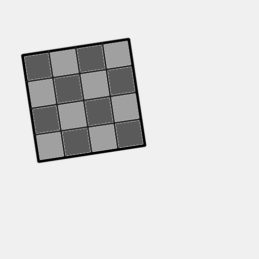
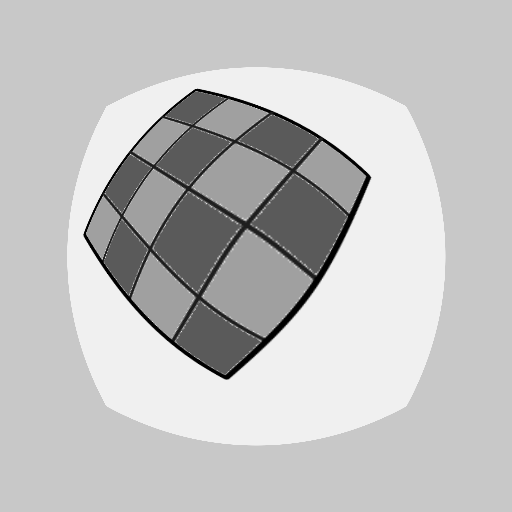
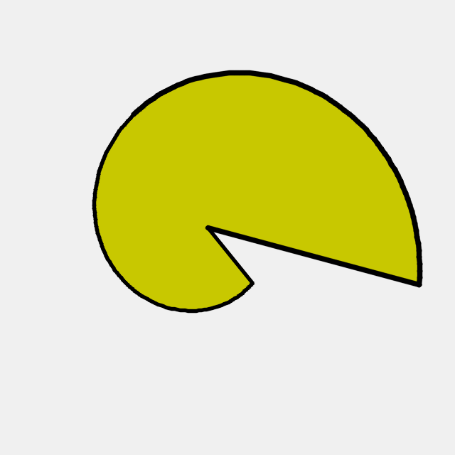
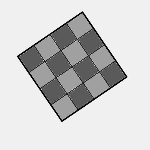
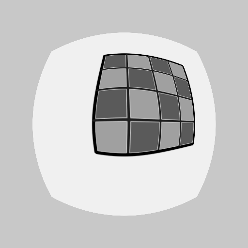
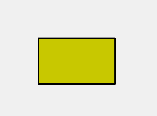
A set of synthetic test cases was used to validate the model mathematics and debug its implementation. Four models were used: upright rectangle, 4X4 checkerboard, distorted 4X4 checkerboard, and a spiral sector:
| upright rectangle | 4X4 checkerboard | distorted 4X4 grid | spiral sector |
|---|---|---|---|
 |
 |
 |
 |
 |
 |
 |
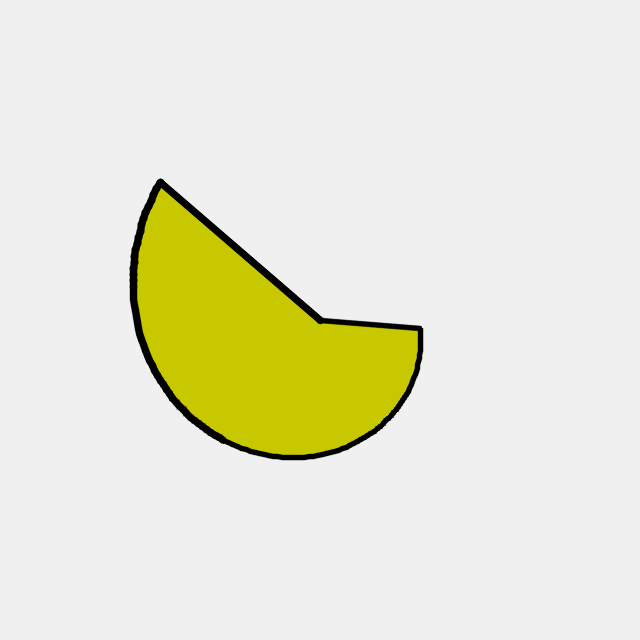 |
These model were selected to address various detection aspects:
1) Upright rectangle is defined by its center, width, height, and edge width. It has detectable internal pattern / color. At high quality input, detecting UR looks trivial; it is enough to analyze the evidence projection on the X and Y axis. It becomes more challenging as the quality decreases...
2) 4X4 checkerboard is defined by its center, width, angle, and edge width. It has an internal pattern of alternating color.
3) Distorted 4X4 checkerboard is similar to the 4X4 checkerboard above, with additional barrel distortion, which changes the polar coordinates \(\{R, \theta\}\) of each point to \(\{R_d, \theta\}\): $$ R_d = (1+\frac{L_0}{L_f})*\frac{R}{1 + R/L_f} $$ where \(L_f\) is an unknown distortion parameter; the smaller it is, the stronger is the distortion. \(L_0\) is a known constant using for stretching the resulting image; here it was set to 1/4 the image width. Detecting the object requires detection of \(L_f\) as well.
4) Spiral sector is a sector of a logarithmic spiral, defined by its center, orientation \(\theta_0\), starting radius \(R_0\), angular span \(\Theta\), and growth exponent \(b\). Its polar coordinates relative to its center are given by:. $$ r(\alpha) = R_0 * e^{b(\alpha- \theta_0)} $$ $$ \theta_0 <= \alpha <= \Theta + \theta_0 $$ The object has detectable internal pattern / color.
Test scheme:
For each case, a variety of objects was created programatically, using a wide range of parameters. Each object was used to programmatically create two sets of evidence - edge elements and area elements, with variable amounts of noise, scatter and occlusion; noise are evidence uncorrelated to the object, scatter is the inaccuracy of object evidence, and occlusion are missing evidence.
This test policy, of creating the evidence programatically instead of detecting it in images, is necessary to avoid dependency on edge detection specifics or any other preprocessing steps, and focuses the test on ORCEA unique contribution.
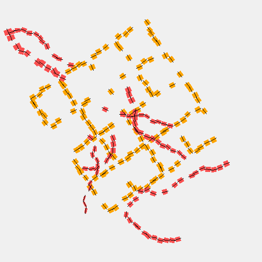
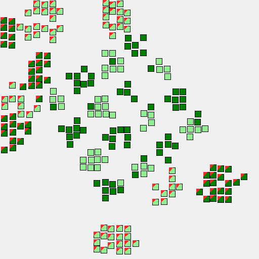
The images below demonstrate how edge elements and area elements are visualized in this work:
- Edge elements have direction and thickness; noise ones are shown in red.
- Noise area elements have red corner.
- In case area elements represent several 'classes' (for examle dark vs. light patches), their color is used to show their classes. See the checkerboard below: light green stands for the dark squares, and dark green for the light squares. In order to make the test more reallistic, some area elements were randomly assigned the wrong class.
| Theoretic object | Edge elements | Area elements (2 classes) |
|---|---|---|
|
 |
 |
Test results
General note:
Tests were conducted using various levels of noise, scatter and occlusion. The Detection rates for meduim and low quality input were > 98% and > 95% respetively; the more interesting tests are the ones using low quality input, as they stretch ORCEA ability to its limits. Where possible, quality was degraded radically in order to find at what conditions detection goes below 80%.
 Upright rectangle
- High quality example:
-
There is little noise and scatter; ORCEA requires only 25 evidence to converge
- Medium quality (more noise and scatter):
-
Takes ~45 steps to converge, with some fluctuations starting around step 30
- Low quality:
-
Convergeance starts after 180 steps
- Unusable edge elements, high quality area elements:
-
Massive noise, edge elements nearly useless. Takes 350 steps to achieve convergeance.
In this case area elements contribute more to detection than edge elements
A link to full test results will be added.
4X4 checkerboard
- High quality example:
-
There is little noise and scatter; ORCEA requires only 45 pieces of evidence to converge
- Low quality sample:
-
Takes ~90 steps to converge
- No edge elements (beside noise):
-
Slow convergeance that starts only after 140 steps.
- No edge elements (beside massive noise):
-
Massive noise edge elements. Convergeance only towards the end.
In this case area elements contribute more to detection than edge elements - Massive noise of area elements:
-
Massive noise area elements throw ORCEA off-balance until step 169, where enough edge elements were accumulated.
In this case ORCEA sucseeds to ignore the massive area elements noise .
A link to full test results will be added.
Spiral sector
- Low quality input:
-
Example with low-quality evidence
- Low quality edge element:
-
Example with only low-quality edge elements
Distorted 4X4 checkerboard
Coming soon...